Rainfall pattern in Kumasi, Ghana

This post illustrates R’s ability to draw a follow-up plot, isolating one period so it can be compared to the other.

dataD <- 
    readxl::read_excel("C:\\Dataset\\rainfall.xlsx")

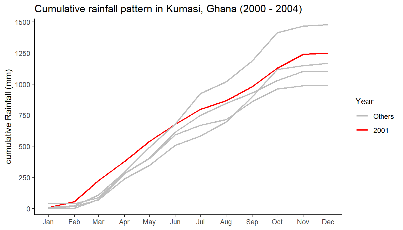
the_year <- 2001
dataD %>% 
    janitor::clean_names() %>% 
    rename(date_1 = time) %>% 
    arrange(date_1) %>% 
    mutate(year_1 = lubridate::year(date_1),
           day = lubridate::day(date_1), 
           mth = lubridate::month(date_1),
           the_year = year_1 == the_year) %>%
    group_by(year_1) %>% 
    mutate(cum_rainfall = cumsum(rainfall)) %>% 
    ungroup() %>% 
    mutate(
        new_date = lubridate::ymd(str_glue("2000-{mth}-{day}"))) %>% 
    ggplot(aes(x = new_date, y = cum_rainfall, 
               group = year_1)) +
    geom_line(aes(col = the_year),linewidth = 0.8) +
    labs(y = "cumulative Rainfall (mm)", 
         title = "Cumulative rainfall pattern in Kumasi, Ghana (2000 - 2004)")+
    scale_x_date(name = NULL,date_breaks = "1 month",date_labels = "%b") +
    scale_color_manual(name = "Year", 
                       labels = c("Others", the_year), 
                       values = c("grey","red"))+
    scale_size_manual(breaks = c(F,T), values = c(0.5,0.7), guide = "none")+
    scale_y_continuous(breaks = seq(0,1500, 250), expand = c(0,50)) +
    theme_classic()